Many languages exist to model the structure of data. Well-known examples include Entity-Relationship Diagram (ERD) by Chen, UML class diagrams and the Object-Role Modeling (ORM) language. Each notation has its own graphical notation. To model constraints additional languages are required. For example, the Object Constraint Language (OCL) can be used for UML class diagrams. However, the basics of data modeling resides in set theory and first-order logic.

In this tutorial, we explain a simple approach to represent data models using set theory, and show how constraints can be expressed in first-order logic. The approach comes with a simple tool to assist the modeler. The tool can be downloaded here.

First, we start with some basic notions in logic and set theory, after which we will dive into a data modeling assignment.

Some basics in logic

Set theory

Before we start modeling, first a small crash course on set theory and logic. A set is nothing more than a collection of elements. If the sets are finite, we can visualize the elements using a Venn-Diagram. An example is depicted below.

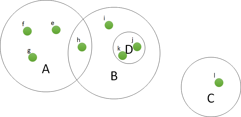
The Venn diagram shows four sets, named A, B, C, and D. All elements together form the universe, U. Some elements can be part of multiple sets. For example, element h belongs to sets A and B, and elements k and l reside in both B and D. Formally, we write this universe as follows:

$\begin{array}{lcl} Universe & = & \{ e, f, g, h, i, j, k, l \} \\ A & = & \{e, f, g, h \}\\ B & = & \{ h, i, j, k \} \\ C & = & \{ l \} \\ D & = & \{ j, k \} \\\end{array}$

On the universe, we can make statements. First a simple one, to state that an element resides in some set. For example, to write that e resides in A, we write:

$e \in A$

A common statement is the union of A and B, which are all elements that reside in A, B or both. Formally:

$A \cup B = \{ e, f, g, h, i, j, k \}$

The intersection of A and B are all elements that reside both in A and in B, in our example only h. Formally:

$A \cap B = \{ h \}$

The difference of a set with some other set are all elements that are in the former, but not in the latter. For example, the difference of A with B are the elements e, f, and g. Formally we can write this in set theory as:

$A \setminus B = \{ e, f, g \}$

A subset is a set that fully resides in some other set. Consider for example sets B and D. Then, any element that resides in D, also resides in set B. Hence, D is a subset of B. There are two ways to write this formally. The first is in set theory:

$D \subseteq B = \{ j, k \}$

The second notation is in first-order logic: for all elements in the universe, it is true that if x is in D, then it is also in B. Formally:

$\forall x \in \mathrm{U} : (x \in D) \implies (x \in B)$

With first order logic, one can make all kinds of statements. For example, one can state that the intersection of A and B is not empty. To formalize this in first-order logic, we rewrite the statement into: there exists an element that is in both A and B. Which can be formalized as:

$\exists x \in \mathrm{U} : (x \in A) \wedge (x \in B)$

Similarly, we can state that the intersection of B and C is empty, by stating that no element exists that is in both:

$\neg ( \exists x \in \mathrm{U} : (x \in B) \wedge (x \in C) )$

By applying De Morgan, one can rewrite the statement:

$\forall x \in \mathrm{U} : \neg ( (x \in B) \wedge (x \in C) )$

Statements need not to be valid in a universe. For example, the statement that there exists an element in the intersection of B and C, does not hold in this universe. To prove this statement, one needs to search for an element such that the latter part of the formula is true. In this case, this is not true: such an element does not exist. The first statement, that the intersection of A and B is not empty, is true, as the statement holds for element h. To prove a universal quantifier, one needs to show that the statement holds for any element in the universe. Such proofs can become very tedious.

Tool support

To support the modeler in validating a universe, we developed a tool. It uses the TFF notation that is used for many automated theorem provers. The above universe can be formalized as follows:

  tff( e_in_universe, type, e: universe ).
  tff( f_in_universe, type, f: universe ).
  tff( g_in_universe, type, g: universe ).
  tff( h_in_universe, type, h: universe ).
  tff( i_in_universe, type, i: universe ).
  tff( j_in_universe, type, j: universe ).
  tff( k_in_universe, type, k: universe ).
  tff( l_in_universe, type, l: universe ).

Each line follows the following syntax: first we inform that we add a “clause” in tff format. Next is the name (which should be unique). We specify the elements and their type, which is given by the second parameter. The third parameter defines the element, and its type (universe). Any name for the elements and types can be used, as long as they start with a lower letter, and only contain letters and digits.

TFF is based on axioms and conjectures. An axiom is a given statement, a clause that is assumed to be true. A conjecture is a statement that we need to proof to be correct. We use axioms to define sets and their elements, and conjectures to add statements on those sets. In TFF-format, the sets in the Venn-diagram look like this:

  tff( e_in_A, axiom, a(e) ).
  tff( f_in_A, axiom, a(f) ).
  tff( g_in_A, axiom, a(g) ).
  tff( h_in_A, axiom, a(h) ).
  tff( h_in_B, axiom, b(h) ).
  tff( i_in_B, axiom, b(i) ).
  tff( j_in_B, axiom, b(j) ).
  tff( k_in_B, axiom, b(k) ).
  tff( l_in_C, axiom, c(l) ).
  tff( j_in_D, axiom, d(j) ).
  tff( k_in_D, axiom, d(k) ).

Notice that we use small letters for the sets as words starting with a capital are interpreted as variables. Last, we write our statements as conjectures on the above universe. For the statement

$\exists x \in \mathrm{U} : ( x \in B \wedge x \in C )$ thus becomes:

  tff( intersection_b_c_not_empty, conjecture,
      ? [X: universe ] : 
        ( 
            b(X) & c(X) 
        )
  ).

The above statement shows that we want to prove a conjecture. We use ? for the existential quantifier, and & for the and operator. Similarly, we can translate the statement of D being a subset of B by using the ! for the universal quantifier, and => for the implication:

  tff( d_is_a_subset_of_b, conjecture,
    ! [X: universe ] : 
      (
          ( d(X) ) => ( b(X) )
      )    
  ).

The complete example can be downloaded here. Once the file is fed to the tool, the tool starts to prove the conjectures. The conjectures it cannot prove are printed on the command line. If all goes well, the following output is generated:

$ java -jar Prover.jar example1.tff
I could not find a proof for the following conjectures:
 *  intersection_b_c_not_empty

To get an explanation of why the tool cannot find a proof for the conjecture, run the following command:

$ java -jar .\Prover.jar --explain example1.tff
I could not find a proof for the following conjectures:
* intersection_b_c_not_empty is not valid
  Explanation:
    Because:
     ( ! [ X: universe ] : ( ~( ( b( X)& c( X) ) ) ) )
    Hence:
      Not( intersection_b_c_not_empty )

The tool states that for all elements in the universe no element X can be found such that b(X) and c(X). Hence, the intersection is empty.

Relations

Elements can have relations. For example, if elements resemble persons, a relation can be that one person likes some other person, or that one person is married to some other person. To explain relations, we start with the cartesian product. The cartesian product is defined between two sets, and denotes that any element in the former set is related to all elements in the latter. Formally:

$A \times B = \{ (a,b)\ |\ a \in A \wedge b \in B \}$

In the above case, the cartesian product of A and D results in the following set:

$A \times D = \{ (e,j), (e,k), (f,j), (f,k), (g,j), (g,k), (h,j), (h,k) \}$

Formally, relations are a subset of the cartesian product. If the relation equals the cartesian product, the relation is called total. However, this is rarely the case. Suppose in our example, A resembles wagons, and B represents locomotives, with D the set of steam engines. Each wagon is coupled to at most one locomotive. Suppose relation coupled depicts this phenomenon:

$\forall a \in A, b,c \in B : (couples(a,b) \wedge couples(a,c)) \implies b = c$

The above statement expresses that if a is coupled to both b and c, then b and c must be equal. A relation that fulfills the above statement is called a function. Similarly, we want that all wagons are coupled to some engine:

$\forall a \in A: \exists b \in B : couples(a,b)$

If this is the case, the relation is called total.

Other often used properties on relations include

symmetry:
$\forall a,b \in A: R(a,b) \implies R(b,a)$
Reflexivity:
$\forall a \in A: R(a,a)$
Transitivity:
$\forall a, b, c \in A : ( R(a,b) \wedge R(b,c) ) \implies R(a,c)$

Sets and relations form the basic building blocks of any data modeling technique.

Tool support

In the tool, we can specify relations as follows. We follow the example above that wagons are coupled to engines. We write this as axioms in TFF-format:

  tff (e_coupled_to_j, axiom, coupled(e, j) ).
  tff (f_coupled_to_j, axiom, coupled(e, j) ).
  tff (g_coupled_to_k, axiom, coupled(e, j) ).
  tff (h_coupled_to_j, axiom, coupled(e, j) ).

Next, we can state our conjectures, that coupled should be a total relation:

  tff ( coupled_is_total, conjecture,
    ! [Wagon : universe ] : 
      (
        ( a( Wagon ) ) => ( ? [ Engine : universe ] : ( d( Engine ) & coupled(X,Y) )  )
      )
  ).

And that coupled should be a function:

  tff ( coupled_is_a_function, conjecture,
    ! [Wagon : universe, Engine1: universe, Engine2: universe ] : 
      (
        ( coupled(Wagon, Engine1) & coupled(Wagon, Engine2) )
        =>
        ( Engine1 = Engine2 )
      )
  ).

This concludes the basic notions required to understand sets and relations to model the structure of data, and constraints on the structure.

Let us consider a last example. Suppose we have a world of males and females, together with a likes relation, as the picture below shows.

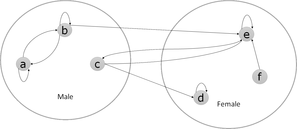
The picture can be easily translated into a universe. Each node becomes an element, and each arc a relation. This leads to the following set of relations (in TFF-notation):

tff( a_likes_a, axiom, likes(a,a) ).
tff( a_likes_b, axiom, likes(a,b) ).
tff( b_likes_b, axiom, likes(b,b) ).
tff( b_likes_a, axiom, likes(b,a) ).
tff( b_likes_e, axiom, likes(b,e) ).
tff( c_likes_d, axiom, likes(c,d) ).
tff( c_likes_e, axiom, likes(c,e) ).
tff( c_likes_c, axiom, likes(c,c) ).
tff( d_likes_d, axiom, likes(d,d) ).
tff( e_likes_e, axiom, likes(e,e) ).
tff( e_likes_c, axiom, likes(e,c) ).
tff( f_likes_e, axiom, likes(f,e) ).

Now, we can create the statement: somebody only likes somebody if they feel good. Translating the statment “feel good” as “likes themselves”, we get the following formalisation:

$\forall X, Y \in Male \cup Female : likes(X,Y) \implies likes(X,X)$

Or, in TFF-notation:

tff( likes_only_if_feels_good, conjecture, 
    ! [X: human, Y: human ] : likes(X, Y) => likes(X, X)
).

Checking this conjecture on the above universe, results in the following explanation by the tool:

$ java -jar .\Prover.jar --explain likesExample.tff
I could not find a proof for the following conjectures:
* likes_only_if_feels_good is not valid
  Explanation:
    Because:
     ( likes( f, e)& ~( likes( f, f) ) )
    Hence:
     ~( ( likes( f, e) => likes( f, f) ) )
    Hence:
     ~( ( ! [ Y: universe ] : ( ( likes( f, Y) => likes( f, f) ) ) ) )
    Hence:
     ~( ( ! [ X: universe ] : ( ( ! [ Y: universe ] : ( ( likes( X, Y) => likes( X, X) ) ) ) ) ) )
    Hence:
      Not( likes_only_if_feels_good )

The output reads as follows: because f likes e, but there is no likes(f, f) relation, it cannot prove the implication, and hence not the for-all statement. The full file of the example can be found here.

A Model Railway Example

Let us consider a larger example. Someone playing with model railways wants to build a software tool to support the driving of trains on its layout. The software system only needs to support a single layout.

A layout consists of tracks that are connected. A station is a set of tracks, as is a switch. Trains run on over a section, which is a collection of tracks.

First version

A first data model is shown in ERD notation below. We assume that each switch has at least one track, and each track belongs to at most one track. Similarly, each station has at least one track, and each track belongs to at most one station. In our first attempt, we do the same for sections, which results in the data model below.

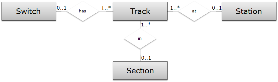
We can translate this model in TFF notation as follows:

  tff( t_a_track  , axiom, track(t)   ).
  tff( w_a_switch , axiom, switch(w)  ).
  tff( s_a_station, axiom, station(s) ).
  tff( p_a_section, axiom, section(p) ).
  tff( w_has_t    , axiom, has(w, t)  ).
  tff( t_at_s     , axiom, at(s, t)   ).
  tff( t_on_p     , axiom, on(t, p)   ).

Next, we can add the constraint. First, we model the domain constraints:

  tff( has_domain, conjecture, 
    ! [W: universe, T: universe ] :
      (
        ( has(W, T) )
        =>
        ( track(T) & switch(W) )
      )
  ).

And next the cardinality constraints:

  tff( each_track_at_most_one_switch, conjecture,
    ! [X: universe, Y1: universe, Y2: universe ] : 
      (
        ( has(X, Y1) & has(x, Y2) )
        =>
        ( Y1 = Y2 )
      )
  ).
  tff( each_switch_at_least_one_track, conjecture, 
    ! [W: universe ] : 
    (
        ( switch(W) )
        =>
        ( ? [T: universe ] : ( has(W, T) )  )
    )
  ).

We repeat this for each relation in the data model. As a next step, we can start populating our data model to validate our assumptions on the relations.

Populating the model

To validate our model, we draw a simple model railway, with two double tracked stations. We have two trains, moving from one station to the other. For this, we define two sections, p1 and p2. The figure below depicts our railway.

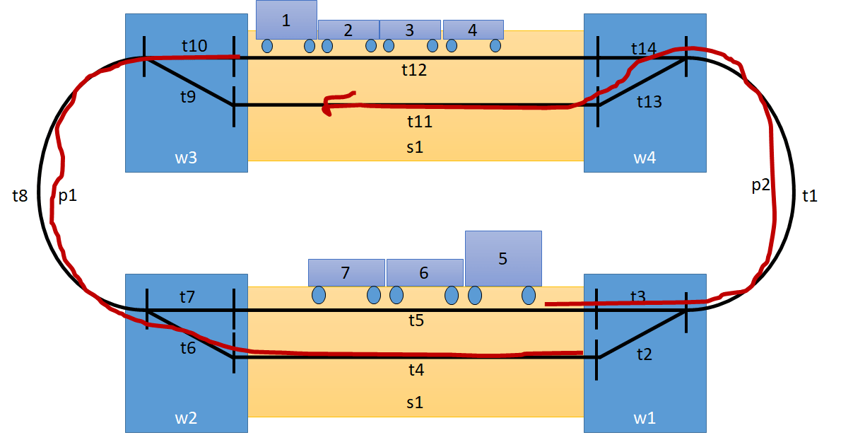
The population then looks as follows:

$\begin{array}{lcl} track & = & \{ t_1, \ldots, t_{14} \} \\ switch & = & \{ w_1, w_2, w_3, w_4 \} \\ station & = & \{ s_1, s_2 \} \\ section & = & \{ p_1, p_2 \}\\ \end{array}$

And each of the relations is populated:

$\begin{array}{lcl}has & = &(\{w_1\} \times \{t_2, t_3\} ) \cup (\{w_2\} \times \{ t_6, t_7 \} ) \\ & \cup & (\{w_3\} \times \{t_9,t_{10}\} ) \cup (\{w_4\} \times \{ t_{13},t_{14}\} ) \\ at & = & ( \{t_4, t_5\} \times \{s_1\} ) \cup ( \{t_{11},t_{12}\} \times \{s_2\} ) \\ on & = & ( \{t_{12}, t_{10}, t_8, t_6, t_4\} \times \{p_1\} ) \\ & \cup & ( \{t_5, t_3, t_1, t_{13}, t_{11}\} \times \{p_2\} ) \\\end{array}$

Next, we represent the universe in TFF-format for our tool, and validate it. The file can be found here. We feed the file to the tool, and all constraints turn out to be valid! Hence, we should be happy…

A second version

But, are we happy? Let us consider the model again. We have a train moving over section p1 from station A to station B. Suppose we define a third section to move the train back to station B, and call this section p3. This track looks as follows:

$\{p_3\} \times \{ t_4, t_2, t_1, t_{14}, t_{12} \} \subseteq on$

But then tracks t4 and t12 are on two sections, which is not allowed by one of the cardinality constraints. Extending our universe with this additional population results in the next TFF-file. Feeding it to our tool, we see that the constraint ‘track_on_at_most_one_section’ is violated. Asking for an explantion, the tool gives the following output:

$ java -jar .\Prover.jar --explain modelRailwayExample2.tff
I could not find a proof for the following conjectures:
* each_track_at_most_one_section is not valid
Explanation:
Because:
( ( on( t12, p1) & on( t12, p3) ) & ~( ( p1 = p3 ) ) )
Hence:
~( ( ( on( t12, p1) & on( t12, p3) ) => ( p1 = p3 ) ) )
Hence:
~( ( ! [ Y2: universe ] : ( ( ( on( t12, p1) & on( t12, Y2) ) => ( p1 = Y2 ) ) ) ) )
Hence:
~( ( ! [ Y1: universe ] : ( ( ! [ Y2: universe ] : ( ( ( on( t12, Y1) & on( t12, Y2) ) => ( Y1 = Y2 ) ) ) ) ) ) )
Hence:
~( ( ! [ X: universe ] : ( ( ! [ Y1: universe ] : ( ( ! [ Y2: universe ] : ( ( ( on( X, Y1) & on( X, Y2) ) => ( Y1 = Y2 ) ) ) ) ) ) ) ) )
Hence:
Not( each_track_at_most_one_section )

Again, the first line directly gives the hint: it found for track t12 to different sections, being p1 and p3, and those are not equal. The counter example shows us to relax the cardinalities for the on-relation between Track and Section. Hence, we update our model, and state that a track can be on any number of sections. In other words, we remove the constraint ‘track_on_at_most_one_section’. This results in the following data model:

On this data model, all constraints are satisfied, and we can add different sections for trains.

Conclusion

This concludes our small tutorial. We hope that this tutorial shows how set theory and first-order logic can aid to build better models. It requires creativity to come up with a suitable data model, but requires rigor to validate whether the model is indeed a good model for the given situation. This requires practice. Tools like our prover assist the modeler in checking the constraints on given populations. However, finding the right populations, as this example shows, remains a tedious and creative process.

Downloads

Prover
Example1 on set theory and relations
likesExample on relations and properties
modelRailwayExample1.tff containing the first version with two sections
modelRailwayExample2.tff containing the first version with three sections

A tutorial on data modeling with sets and first-order logic

Architecture mining

A tutorial on data modeling with sets and first-order logic

Some basics in logic

Set theory

Tool support

Relations

Tool support

A Model Railway Example

First version

Populating the model

A second version

Conclusion

Downloads

Related

Some basics in logic

Set theory

Tool support

Relations

Tool support

A Model Railway Example

First version

Populating the model

A second version

Conclusion

Downloads

Share this:

Related